Your Task for This Lab Is to Read a Data File Containing Star Information
1A: Lab two
Pre-class activities
There are eight activities in total for this pre-class, simply don't worry, they are broken down into very small steps!
Activity 1: Create the working directory
If you want to load data into R, or save the output of what you've created (which y'all almost always will want to practice), y'all first need to tell R where the working directory is. All this means is that we tell R where the files nosotros demand (such as raw data) are located and where we want to salve whatever files you have created. Think of it just like when you have different subjects, and you take split up folders for each topic e.one thousand. biology, history and so on. When working with R, it's useful to have all the information sets and files you need in ane folder.
Nosotros recommend making a new binder called "Psych 1A" with sub-folders for the tutorial and data skills secctions of the labs and saving any slides, activities, data, scripts, and homework files in these folders. We suggest that you lot create these folders on the Grand: drive. This is your personal area on the University network that is condom and secure so it is much better than flashdrives or desktops.
Figure 2.1: Folder structure
- Cull a location for your lab work and then create the necessary folders.
Whatsoever yous do, do Non call the folder you shop your R work in "R". You don't have to telephone call information technology Data Skills, only if you phone call it simply R and then R will have an existential crunch about saving into itself and yous will notice that y'all have problems reading and saving your files.
Activity 2: Fix the working directory
In one case yous have created your folders, open up R Studio. To set the working directory click Session -> Fix Working Directory -> Cull Directory and then select the Data Skills folder as your working directory.
R Markdown for lab piece of work and homework assignments
For the lab work and homework you will use a worksheet format called R Markdown (abbreviated every bit Rmd) which is a great way to create dynamic documents with embedded chunks of code. These documents are self-independent and fully reproducible (if you have the necessary data, you should be able to run someone else's analyses with the click of a push button) which makes it very piece of cake to share. This is an important part of your open science training as ane of the reasons we are using R Studio is that it enables us to share open and reproducible information. Using these worksheets enables you to keep a record of all the lawmaking you lot write during the labs, and when it comes fourth dimension for the portfolio assignments, we can give you a task you can so fill in the required code.
For more information about R Markdown feel gratis to take a look at their primary webpage one-time http://rmarkdown.rstudio.com. The key reward of R Markdown is that it allows y'all to write lawmaking into a document, along with regular text, and then knit information technology using the bundle knitr to create your document equally either a webpage (HTML), a PDF, or Word certificate (.docx).
Activity 3: Open and save a new R Markdown certificate
To open a new R Markdown document click the 'new particular' icon and then click 'R Markdown'. You lot will be prompted to give it a title, call it "Lab 2 pre-class". Also, modify the author name to your GUID every bit this will be good exercise for the homework. Keep the output format every bit HTML.
In one case you've opened a new document be sure to salve it by clicking File -> Salvage equally. You should likewise name this file "Lab ii pre-course". If you've prepare the working directory correctly, yous should now see this file appear in your file viewer pane.
Figure two.2: Opening a new R Markdown certificate
Activity 4: Create a new code chunk
When you first open a new R Markdown document you will encounter a agglomeration of welcome text that looks similar this:
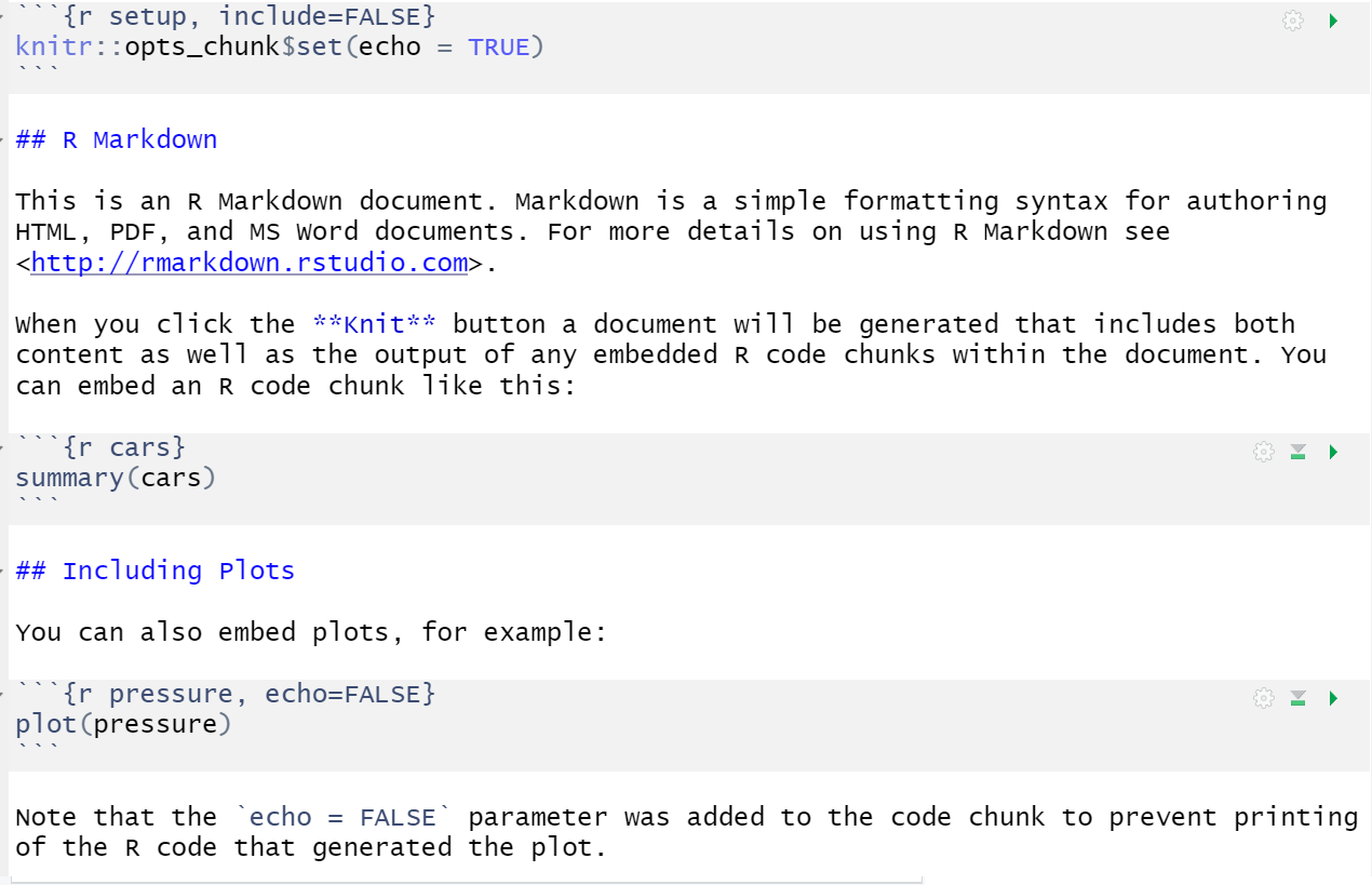
Figure 2.3: New R Markdown text
Practice the following steps:
* Delete everything beneath line 7
* On line viii blazon "About me"
* Click Insert -> R
Your Markdown document should at present look something similar this:
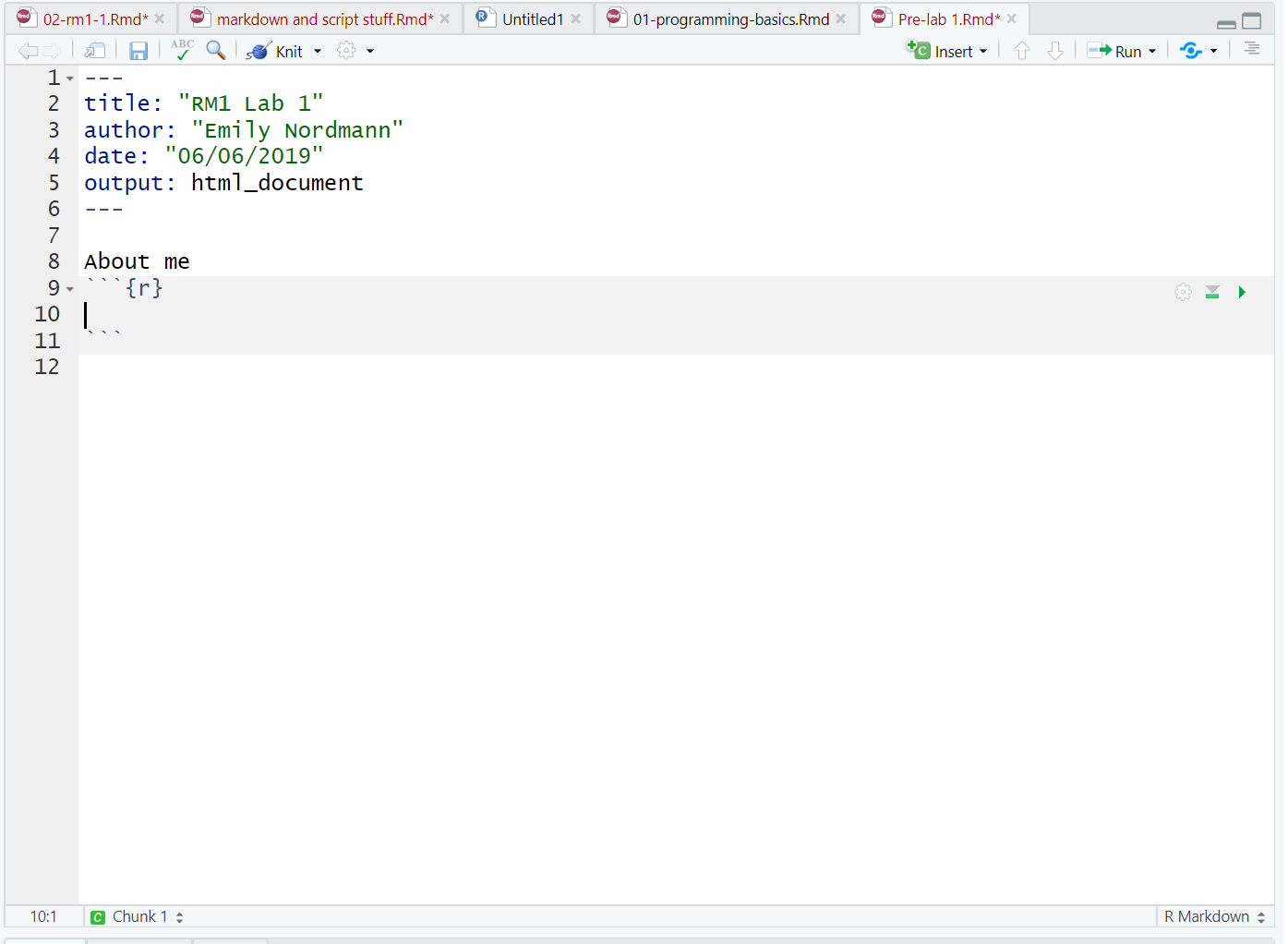
Figure 2.iv: New R chunk
What you have created is a code clamper. In R Markdown, annihilation written in the white space is regarded equally normal text, and anything written in a greyness code chunk is assumed to exist code. This makes it easy to combine both text and lawmaking in one certificate.
When you create a new code clamper you should discover that the grey box starts and ends with three back ticks ```. One common error is to accidentally delete these back ticks. Retrieve, code chunks are grey and text entry is white - if the colour of certain parts of your Markdown doesn't await right, check that you haven't deleted the back ticks.
Activity 5: Write some lawmaking
Now we're going to apply the lawmaking examples y'all read about in Lab i to add some simple code to our R Markdown document.
- In your code chunk write the below code just replace the values of name/age/altogether with your own details).
- Note that text values and dates need to be contained in quotation marks just numerical values do not. Missing and/or unnecessary quotation marks are a common crusade of code not working - remember this!
proper noun <- "Emily" age <- 34 today <- Sys.Date() next_birthday <- as.Date("2020-07-11") Running lawmaking
When you're working in an R Markdown document, there are several ways to run your lines of code.
First, you lot can highlight the lawmaking you lot desire to run and and then click Run -> Run Selected Line(s), nonetheless this is very boring.
Figure 2.5: Irksome method of running code
Alternatively, you can printing the green "play" button at the peak-right of the code chunk and this volition run all lines of lawmaking in that chunk.
Figure 2.6: Slightly better method of running code
Fifty-fifty better though is to learn some of the keyboard shortcuts for R Studio. To run a single line of code, make sure that the cursor is in the line of code yous want to run (it tin can be anywhere) and press ctrl + enter. If you desire to run all of the lawmaking in the code chunk, press ctrl + shift + enter. Learn these shortcuts, they volition make your life easier!
Activity six: Run your lawmaking
Run your code using ane of the methods above. Yous should see the variables name, age, today, and next_birthday appear in the environs pane.
Activity 7: Inline code
An incredibly useful feature of R Markdown is that R can insert values into your writing using inline code. If you've ever had to copy and paste a value or text from one file in to some other, you'll know how easy it can be to make mistakes. Inline code avoids this. Information technology'southward easier to show you what inline lawmaking does rather than to explicate it so let'due south have a go.
First, re-create and paste this text exactly (do not modify anything) to the white space underneath your code chunk.
My proper noun is ` r proper name ` and I am ` r age ` years former. Information technology is ` r next_birthday - today ` days until my birthday. Activity 8: Knitting your file
Nearly finished! As our terminal pace we are going to "knit" our file. This simply ways that we're going to compile our code into a document that is more presentable. To do this click Knit -> Knit to HMTL. R Markdown will create a new HTML document and it volition automatically salve this file in your working directory.
Equally if by magic, that slightly odd bit of text you copied and pasted now appears as a normal sentence with the values pulled in from the objects you created.
My proper noun is Emily and I am 34 years quondam. Information technology is -19 days until my birthday.
Nosotros're not going to apply this function very frequently in the balance of the course merely hopefully yous can see just how useful this would be when writing up a report with lots of numbers! R Markdown is an incredibly powerful and flexible format - this volume was written using it! If you want to push yourself with R, additional functions and features of R Markdown would exist a good place to outset.
Before nosotros terminate, in that location are a few final things to note near knitting that will be useful for the homework:
- R Markdown volition only knit if your lawmaking works - this is a good way of checking for the portfolio assignments whether you lot've written legal lawmaking!
- Y'all can cull to knit to a Word certificate rather than HTML. This can exist useful for e.g., sharing with others, however, it may lose some functionality and it probably won't look as good and then nosotros'd recommend always knitting to HTML.
- You tin can choose to knit to PDF, however, this requires an LaTex installation and is quite complicated. If you lot don't already know what LaTex is and how to use information technology, do non knit to PDF. If you do know how to utilize LaTex, yous don't need us to give you instructions!
- R will automatically open up the knitted HTML file in the viewer, however, y'all tin also navigate to the folder it is stored in and open the HTML file in your spider web browser (east.one thousand., Chrome or Firefox).
Finished
And you're done! On your very first time using R you've not only written functioning code only you've written a reproducible output! You could send someone else your R Markdown certificate and they would be able to produce exactly the aforementioned HTML document every bit y'all, just by pressing knit.
The key matter we want y'all to accept abroad from this pre-form is that R isn't scary. It might be very new to a lot of you, but we're going to take you through it pace-by-step. You'll be amazed at how quickly you can start producing professional person-looking data visualisations and analysis.
In-grade activities
Activity ane: APA referencing
Look at the following reference and reply the below questions:
Smith, M. K., Wood, W. B., Adams, W. Chiliad., Wieman, C., Knight, J. Yard., Guild, N., & Su, T. T. (2009). Why peer discussion improves student functioning on in-grade concept questions. Science, 323(5910), 122-124. https://doi.org/ten.1126/science.1165919
- How many authors are at that place?
- What is the name of the journal?
- How many pages is the commodity?
According to APA style:
- The championship of the paper should be .
- When using a direct in-text citation yous should use to connect the names of the authors.
- When citing a paper with multiple authors, if there are more than ii authors the offset time y'all cite the newspaper in the essay y'all should
Et al means and others. It'southward a common academic phrase that's used when referring to piece of work with more than iii authors.
Data skills
Part of becoming a psychologist is asking questions and gathering data to enable you to answer these questions effectively. Information technology is very important that you sympathize all aspects of the research procedure such equally experimental design, ethics, data management and visualisation.
In this course, you lot will continue to develop reproducible scripts. This means scripts that completely and transparently perform an analysis from first to finish in a way that yields the same result for different people using the same software on different computers. And transparency is a key value of science, every bit embodied in the "trust but verify" motto. When you lot do things reproducibly, others can sympathize and cheque your piece of work.
This benefits science, but at that place is a selfish reason, too: the near important person who will do good from a reproducible script is your hereafter self. When you lot return to an analysis afterward 2 weeks of vacation, you will thank your earlier cocky for doing things in a transparent, reproducible way, equally y'all tin can easily choice up right where you left off.
As role of your skill development, it is of import that you lot piece of work with information then that you tin can become confident and competent in your direction and analysis of data. In the labs, nosotros will work with real data that has been shared by other researchers.
Getting data ready to work with
Today in the lab you volition learn how to load the packages required to work with our information. Y'all'll then load the data into R Studio before getting it organised into a sensible format that relates to our research question. If you lot can't recollect what packages are, go back and revise 1.1.9.
Activeness 2: Set-up
Before we begin working with the information nosotros need to do some set-upward. If you need assistance with whatever of these steps, you should refer to Chapter 2.1:
- Y'all should have already download the data files every bit office of Activeness 5 in Lab one, however, here they are over again if you need them:
Psych 1A Data Files. Extract the files and so move them in to your Data Skills folder. - Download the
Lab 2 Markdown File, extract it, and move it to your Data Skills binder. - Open R and ensure the environment is clear.
- Set the working directory to your Data Skills folder.
- Open up the
stub-ii.2.Rmdfile and ensure that the working directory is set to your Data Skills folder and that the two .csv information files are in your working directory (yous should run across them in the file pane).
Activeness iii: Load in the bundle
Today we need to utilize the tidyverse package. Y'all will employ this parcel in every unmarried lab on this form equally the functions it contains are those we apply for data wrangling, descriptive statistics, and visualisation.
- To load the
tidyversetype the following code into your code chunk (not the console) and then run it.
Activity 4: Read in data
At present we can read in the data. To do this we will utilise the function read_csv() that allows usa to read in .csv files. In that location are also functions that allow you to read in .xlsx files and other formats, yet in this grade we will only use .csv files.
- First, we will create an object called
datthat contains the data in theahi-cesd.csvfile. And then, we volition create an object calledinfothat contains the data in theparticipant-info.csv.
dat <- read_csv ("ahi-cesd.csv") pinfo <- read_csv("participant-info.csv") There is also a function chosen read.csv(). Be very conscientious Not to utilize this function instead of read_csv() as they have dissimilar ways of naming columns. For the dwelling, unless your results match ours exactly you will not get the marks which means yous need to be careful to utilise the right functions.
Activeness v: Check your data
You should at present see that the objects dat and pinfo have appeared in the environment pane. Whenever you read data into R you should always practice an initial check to see that your data looks like you expected. There are several ways you can do this, endeavor them all out to come across how the results differ.
- In the environment pane, click on
datandpinfo. This will open the data to give you lot a spreadsheet-similar view (although you can't edit it like in Excel) - In the surroundings pane, click the small bluish play button to the left of
datandpinfo. This will show yous the structure of the object information including the names of all the variables in that object and what blazon they are (also seestr(pinfo)) - Use
summary(pinfo) - Employ
head(pinfo) - Only type the name of the object you lot want to view, due east.g.,
dat.
Activeness 6: Bring together the files together
We have two files, dat and info but what we actually want is a single file that has both the data and the demographic information about the participants. R makes this very piece of cake past using the function inner_join().
Call back to apply the help function ?inner_join if you want more than information about how to apply a function and to use tab auto-complete to help y'all write your code.
The below code will create a new object all_dat that has the data from both dat and pinfo and it will use the columns id and intervention to match the participants' information.
- Run this code and so view the new dataset using one of the methods from Action four.
all_dat <- inner_join(x = dat, # the first table you want to join y = pinfo, # the 2d table you desire to join by = c("id", "intervention")) # columns the two tables have in common Activity 7: Pull out variables of interest
Our final stride is to pull our variables of interest. Very frequently, datasets will accept more variables and data than yous actually want to use and it tin make life easier to create a new object with just the data you lot need.
In this case, the file contains the responses to each individual question on both the AHI scale and the CESD scale likewise equally the total score (i.e., the sum of all the individual responses). For our analysis, all we intendance almost is the total scores, also as the demographic information about participants.
To do this nosotros use the select() function to create a new object named summarydata.
summarydata <- select(.data = all_dat, # name of the object to accept information from ahiTotal, cesdTotal, sex, age, educ, income, occasion,elapsed.days) # all the columns you want to keep - Run the in a higher place code and then run
head(summarydata). If everything has gone to plan it should expect something like this:
| ahiTotal | cesdTotal | sex | historic period | educ | income | occasion | elapsed.days |
|---|---|---|---|---|---|---|---|
| 32 | 50 | 1 | 46 | four | 3 | five | 182.03 |
| 34 | 49 | one | 37 | 3 | 2 | 2 | 14.nineteen |
| 34 | 47 | i | 37 | iii | 2 | 3 | 33.03 |
| 35 | 41 | one | xix | ii | 1 | 0 | 0.00 |
| 36 | 36 | ane | forty | 5 | 2 | 5 | 202.ten |
| 37 | 35 | 1 | 49 | 4 | 1 | 0 | 0.00 |
Action 8: Visualise the data
Equally you're going to acquire about more over this course, information visualisation is extremely important. Visualisations can exist used to give you more data almost your dataset, but they tin can besides be used to mislead.
We're going to expect at how to write the code to produce simple visualisations in Lab 3 and Lab 4, for now, we want to focus on how to read and interpret unlike kinds of graphs. Please feel free to play effectually with the lawmaking and alter TRUE to False and adjust the values and labels and come across what happens just practise not worry near understanding the code. Merely copy and paste information technology.
Copy, paste and run the below lawmaking to produce a bar graph that shows the number of female person and male participants in the dataset.
ggplot(summarydata, aes(ten = as.factor(sex), fill = as.factor(sex))) + geom_bar(show.legend = FALSE, alpha = .8) + scale_x_discrete(name = "Sex") + scale_fill_viridis_d(option = "E") + scale_y_continuous(name = "Number of participants")+ theme_minimal() Are in that location more male person or more female participants (you volition need to check the codebook to discover out what i and 2 mean to answer this)?
Copy, paste, and run the below lawmaking to create violin-boxplots of happiness scores for each income group.
ggplot(summarydata, aes(10 = as.gene(income), y = ahiTotal, fill = as.cistron(income))) + geom_violin(trim = FALSE, show.fable = FALSE, alpha = .four) + geom_boxplot(width = .2, bear witness.legend = FALSE, alpha = .7)+ scale_x_discrete(name = "Income", labels = c("Beneath Average", "Boilerplate", "Above Average")) + scale_y_continuous(name = "Authentic Happiness Inventory Score")+ theme_minimal() + scale_fill_viridis_d() - The violin (the wavy line) shows density. Basically, the fatter the wavy shape, the more than data points there are at that point. It'southward called a violin plot because it very often looks (kinda) like a violin.
- The boxplot is the box in the middle. The black line shows the median score in each group. The median is calculated by arranging the scores in order from the smallest to the largest and then selecting the center score.
- The other lines on the boxplot show the interquartile range. In that location is a really good caption of how to read a boxplot hither.
- The black dots are outliers, i.east., extreme values.
Which income group has the highest median happiness score?
Which income group has the lowest median happiness score?
How many outliers does the Average income group accept?
Finally, attempt knitting the file to HTML. And that's information technology, well done! Recall to save your Markdown in your Lab ii folder and brand a annotation of any mistakes you made and how you fixed them.
Finished!
Well done! You have started on your journey to become a confident and competent member of the open scientific customs! To testify united states how competent you are you should now complete the homework for this lab which follows the same instructions every bit this in-class action merely asks yous to work with different variables. Ever use the lab prep materials besides as what you do in grade to assist y'all complete the class assessments!
Debugging tips
- When you downloaded the files from Moodle did you salve the file names exactly as they were originally? If y'all download the file more than once you will observe your computer may automatically add a number to the end of the file name.
information.csvis non the same every bitdata(1).csv. Pay close attention to names! - Have you used the exact same object names as we did in each activity? Remember,
proper nameis different toProper noun. In society to make sure y'all tin follow along with this volume, pay special attention to ensuring you use the same object names as we practise.
- Accept you used quotation marks where needed?
- Take you accidentally deleted whatever back ticks (```) from the get-go or end of code chunks?
Examination yourself
- When loading in a .csv file, which function should you use?
Call up, in this class nosotros use read_csv() and it is important for the homework that you use this office otherwise you may observe that the variable names are slightly different and y'all won't get the marks
- The function
inner_join()takes the arguments10,y,by. What doespastpractice?
- What does the function
select()practice?
Homework instructions
But like you did in the pre-class, we're going to use R Markdown for the homework sheets. If you lot haven't done the pre-class, please work through it before attempting the homework.
At that place are just a couple of important rules we demand you lot to follow to make sure this all runs smoothly.
- These worksheets demand to y'all fill in your answers and not change whatever other data. For example, if we enquire you to supplant NULL with your answer, only write in the code you lot are giving equally your respond and cipher else. To illustrate -
Task 1 read in your data
The task to a higher place is to read in the data file nosotros are using for this job - the correct answer is data <- read_csv(data.csv). Y'all would replace the NULL with:
Solution to Chore one
data <- read_csv("data.csv") This means that we can look for your code and if information technology is in the format we expect to encounter it in, nosotros tin can give you the marks! If y'all decide to go all creative on u.s.a. so we can't requite yous the marks equally 'my_lab_Nov_2018.csv' isn't the filename we have given to you to use. So don't change the file, variable or data frame names as nosotros need these to be consistent.
- We will look for your answers within the boxes which offset and terminate with ``` and accept {r task name} in them e.m.
```{r tidyverse, messages=FALSE}
```
These are called code chunks and are the office of the worksheet that we tin read and pick out your answers. If yous modify these in any way we tin can't read your answer and therefore we tin can't give you marks. You can see in the example above that the code chunk (the grey zone), starts and ends with these back ticks (normally constitute on top left corner of the keyboard). This lawmaking chunk has the ticks and text which makes information technology the part of the worksheet that will incorporate code. The {r tidyverse} function tells us which task information technology is (e.1000., loading in tidyverse) and therefore what we should exist looking for and what nosotros can requite marks for - loading in the package chosen tidyverse in the example to a higher place. If this changes then it won't be read properly, so will touch on your grade.
The easiest way to apply our worksheets is to call back of them as fill up-in-the-blanks and keep the file names and names used in the worksheet the aforementioned. If you are unsure nearly annihilation so utilise the forums on Moodle and Slack to ask any questions and come along to the do sessions.
Homework files
You can download all the R homework files and Cess Information you need from the Lab Homework section of the Psych 1A Moodle. .
Source: https://psyteachr.github.io/ug1-practical/a-lab-2.html
0 Response to "Your Task for This Lab Is to Read a Data File Containing Star Information"
Post a Comment